
VQL is a language for representing queries over xAPI statements and how they should be processed and rendered. It underlies the Veracity Learning LRS in several places, including the xAPI and dashboarding components. There are also a few features that allow you to supply your own VQL to the system, so learning VQL can help you get the most out of the LRS.
VQL represents xAPI statement search, processing and visualization. It's a JSON serialized format, meaning that you'll interact with the server by sending JSON encoded JavaScript objects which adhere to the VQL schema.
The most basic component of VQL is the query.
{
    filter: <a filter object or null>,
    process: [
        <an array of processing stages></an>
    ],
    title:"",
    defs:{}
}
A query has 2 parts, the filter and the process. A query with no process will return raw xAPI statements. A query with no filter will process all data through the requested process. When both a filter and process are defined, the filter will filter the data before the process is applied.
A process is a series of steps that transform the data from the previous step (or all data that passes the filter). Each step in a process is an object with a single property. The name of the property corresponds to the action to take, and the value is an object with the required setting for the action.
{
    filter: {},
    process: [
        {
            $frequentValues:{
                path:"actor.id"
            }
        }
    ],
    title:"",
    defs:{}
}
The above example runs the $frequentValues command over all data in the LRS. Data flows from one command in the process to the next, until reaching the end of the process. The result of the query is the data at this point.
There are several places you can use VQL in the LRS.
A filter is a way to either search for xAPI statements, or to narrow the scope of a process. A basic filter sets conditions for fields on a statement
{
    filter: {
        "actor.id":"mailto:[email protected]"
    },
    process: [
        {
            ...
        }
    ]
}
When a filter contains a property name that matches a xAPI statement path, and the value of that property is basic data type like a string or number, the filter selects statements where the path equals the value. The filter above selects statements where the actor.id is "mailto:[email protected]" (Note that Veracity Learning computes an actor.id field to be the IRI of the agent. See it xAPI spec.)
{
    filter: {
        "actor.id":{
            $in:{
                ["mailto:[email protected]","mailto:[email protected]"]
            }
        }
    },
    process: ...
}
When the value of a path is a complex object, the object must contain a single property from the set of allowed operators. The value of the property is the parameter to the operator. Valid operators are:
You can use special objects to denote the logical and, or, not, concepts. The objects are activated with special properties at the top level of the filter object. Note: when multiple properties are defined outside of a logical operator, they are ANDed together.
{
    filter: {
        "object.id":"https://moodle.com/example",
        "result.completion":true
    },
    process: ...
}
The above filter selects statements where the object.id is "https://moodle.com/example" and result.completion is true.
{
    filter: {
       $or:[
            { "object.id" : "https://moodle.com/example" },
            { "result.completion":true }
       ]
    },
    process: ...
}
The above filter selects statements where the object.id is "https://moodle.com/example" or result.completion is true.
{
    filter: {
       $and:[
            { "timestamp" : {$lt : 1581907990413} },
            { "timestamp" : {$gt : 1581906990413} },
       ]
    },
    process: ...
}
The above filter selects statement with timestamps between 2 values. Note that we must use a top level $and in this case, because JSON object cannot have the same property name twice.
VQL can paginate results so you can select a subset of the matched statements. Note: this only applies when the process is empty. To sort, skip or limit, include top level keys in the filter object like so:
{
    filter: {
      $skip:100,
      $limit:100
    },
    process: ...
}
The above example returns the second "page" of statements, when a page has 100 statements. The skip plus limit numbers must be less than the result query window, which is currently defined at 10,000. If your query returns more than 10,000 results, choose a narrower filter, perhaps by filtering on timestamp or stored.
You can sort the query by providing an object under the $sort key. This object should have property names that are statement paths, and values of either "asc" (for ascending) or "desc" (for descending).
{
    filter: {
      $sort:{
          "result.score.scaled" : "asc"
      }
    },
    process: ...
}
The above filter will return statements in ascending order by the value of result.score.scaled. You can supply a second (and third) key for sorting when there are several statements with equal values at the first key.
{
    filter: {
      $sort:{
          "result.score.scaled" : "asc",
          "stored":"desc"
      }
    },
    process: ...
}
The above filter sorts first by result.score.scaled then on the stored value.
There are several special modifiers that can be added to a filter to change its behavior.
In VQL, the processing is modeled as an array of commands, each one consuming a list of documents and outputting a list of documents. A component called the Planner tries to select the best database to fulfill the list of commands. In some cases, different parts of a process can execute in JavaScript, MongoDB and ElasticSearch, all in the same query. The Planner attempts to order operations to minimize the switching between databases and JavaScript and compute the result in the fastest time. Some commands can only be achieved by a single technology, while others can be run in several. Regardless, results are designed to be the same, so the Planner can freely choose one solution or another. In some cases, your installation may not have a healthy ElasticSearch connection. In this case, the Planner will select a Mongo DB and JavaScript only strategy. While the queries will compute the same results, this can significantly effect performance. Because there is a hard time limit of 10 seconds to complete a query, a healthy ElasticSearch connection may be required to get practical results from large data sets.
When there is no process, VQL imposes a sanity limit of 10000 results. When the query can be fulfilled by a strategy that does not pull statements out of a database, this limit is not enforced, and the entire data set is considered. There are some formulations of VQL that will require statements to be pulled in to JavaScript before processing. In this case, the 10000 statement limit is enforced. Check the output of $explain if you think this might be happening.
The first command in the process takes as its input the list of statements that pass the filter. Usually, this first command can be computed in the DB, and so the 10000 statement limit is not enforced.
In VQL commands, a parameter that expects a statement path always ends with the word "path". It often IS the word "path". These paths should be the simple JSON notation for a path into a statement, like "result.response" or "object.definition.type". You can also use array notation, such as "context.contextActivities.parent[0].id". For extensions, because the keys contain dots, use bracket notation, like "context.extensions['http://www.test.com/extension'].value"
When a statement path is expected by a command that "consumes" a query ( meaning that command uses the query against the statement database), don't include the leading "$". When a command is used in such a way as there are incoming documents, you should use the leading "$", and then the dot notation path. For instance:
{
    filter:null,
    process:[
        {
            $max:{
                path:"result.score.raw"
            }
        }
    ]
}
The above path matches against statements, and the $max stage filters on the whole statement database, since it's the first stage in the process.
{
    filter:null,
    process:[
        {
            $paths:{
                ...
            }
        },
        {
            $max:{
                path:"$duration"
            }
        }
    ]
}
In this case, we use $duration to signal that we are computing against the incoming document stream, rather than the statements themselves.
Many of the most useful commands in VQL support additional query logic by computing "metrics". A "metric" is some value you compute by supplying an operator and a path. All commands that support metrics support the basics
Metrics are named, and all output documents have the name and the corresponding value appended. For instance,
    {
        $timeSeries:{
            path:"timestamp"
        }
    }
This query generally outputs a stream of documents in the form
[
    {
        _id: 2342847019273,
        count: 10
    },
    ...
]
If you request an additional metric, you do so like this:
    {
        $timeSeries:{
            path:"timestamp",
            metrics:{
                averageScore:{
                    $avg:"result.score.raw"
                }
            }
        }
    }
In the above example, the metrics name is 'averageScore', the operator is "$avg", and the path is "result.score.raw". The output document stream will now be
[
    {
        _id: 2342847019273,
        count: 10,
        averageScore: 15.5 //or some computed value
    },
    ...
]
While you can have several named metrics, each metric can have only one operator. Every operator expects it's value to be a path. The word "metrics" above is special - every command that supports metrics expects them to be inside this key. Some commands support special metrics beyond these. The general pattern is the same, but some extended metrics expect complex objects full of settings, rather than just a string path.
VQL includes a set of commands intended to make common operations easy. These commands cover both visualization and data processing, and are written such that the default outputs of the common processing commands match seamlessly with certain rendering commands. See "Rendering" below for more information on rendering visualizations. Every command in the process should be a JSON object with a single property. This property is the command name, which will always start with a '$'. The value of the property is an object containing the necessary command parameters.
{
    filter: null,
    process: [
        "$frequentValues":{
            path: "actor.id"
        }
    ]
}
The above query computes the 10 most common actor IDs.
This command finds the most common N distinct values of some path. It supports metrics and sorting by those metrics.
{
    $frequentValues:{
        path: "actor.id",
        limit:10,
        sort :'<see "sorting">',
        metrics :'<metrics "see metrics">'
    }
}
Like other processing commands, $frequentValues supports metrics. This stage always outputs the count of statements for each unique value, regardless of the metrics configuration.
limit) results are output.Output:
[
    {
        _id:"<the unique value at path>",
        count:"the count of objects with path===_id",
        metrics '<metrics output>'
    }
    ...
]
The resulting document set is an array of objects. The "_id" field of each object is the unique value of the path. Count is the number of times that value occurred.
You can override the selection of values to use some criteria other than the most frequent. You do so by sorting in 'asc' or 'desc' mode on a metric.
{
    "$frequentValues":{
        path:"actor.id",
        metrics:
        {
            score: { $avg: "result.score.scaled" }
        },
        sort:{
            score:"asc"
        }
    }
}
The above process returns the actor.id's with the bottom average scores. Note that we return the 10 (or limit) first results, so sorting in ascending order yields the bottom 10 scores.
You use a slightly special syntax to take the bottom results by count
{
    "$frequentValues":{
        path:"actor.id",
        sort:{
            count:"asc"
        }
    }
}
The above process returns the 10 least frequent actor.ids. Count is a special case metric that is always computed.
In addition to the common types, it supports 2 special case metric types, $timeSeries and $frequentValues. Applying these metrics generates a child data set by splitting all the data that matched each unique value at path and running a $timeSeries or $frequentValues query for just these results.
{
     "$frequentValues":{
        path:"actor.id",
        metrics:{
            topObjects:{
                $frequentValues:{
                    path:"object.id"
                }
            }
        }
    }
}
The above queries computes the top most frequent objects for each of the top most frequent actors. While this can also be computed iteratively in VQL, this representation is easier to understand, and works nicely with the default rendering commands
The output of this command would be
[
    {
        _id: "mailto:[email protected]",
        count: 264,
        topObjects: [
            {
                _id: "http://example.com/mini-game",
                count: 84
            },
            ...
        ]
    },
    ...
]
The above result shows how the output of a metric of type $frequentValues is an array with a similar structure to the outer $frequentValues. Sub $frequentValues and $timeSeries metrics support all the typical configuration as when these commands are used normally. You cannot, however, use these metrics in the sort configuration.
Time series groups data into buckets by day, month or hour according to the value of some path. The datatype of the values at the path should be a timestamp. Generally, the path will be timestamp, but could also be the value of an extension. $timeSeries supports basic metrics, and always includes a default count metric.
{
    $timeSeries:{
        path: "<the path in the statement to a timestamp>",
        span:"either 'daily', 'hourly', or 'monthly'",
        timezone:"a timezone descriptor for selecting month, and day boundaries. Defaults to 'UTC'"
        metrics :'<metrics "see metrics">'
    }
}
Time series supports only the normal metrics. There is no sorting configuration, as data is sorted by time.
{
    $timeSeries: {
            path: "timestamp",
            span: 'daily',
            metrics: {
                score: {
                    $avg: "result.score.scaled"
                }
            }
        },
    },
}
The above command builds a time series for each day, computing the statement count and average of result.score.scaled on each day.
Output
[
    {
        _id: 1560369600000,
        count: 15,
        score: 0.4549999972805381
    },
    ...
]
The $timeSeries command will output a sequence of objects where the _id property is a time in milliseconds, count is the count of statements with a path in that interval, and the metrics specified.
The punchCard command computed a 2D array over a time period, with the outer dimension being days, and the inner being the hours. It computes metrics for each point, and always includes the default count metric. $punchCards are usually rendered with a heat map, but you can also use additional logic to select certain units, for instance, find the busiest day of each month.
{
    $punchCard:{
        path: "<the path in the statement to a timestamp>",
        span:"either 'weekly', or 'monthly'",
        timezone:"a timezone descriptor for selecting month, and day boundaries. Defaults to 'UTC'"
        metrics :'<metrics "see metrics">'
    }
}
As a convenience, a "dayOfWeek" value is returned as well. Note that the special case count is returned for the outer document, while metrics are only computed for the inner.
Output
[
    {
        count: 2199,
        day: 1,
        dayOfWeek: "Monday",
        hours: [
            {
                hour: 0,
                count: 48,
                score: 0.4707142857142857
            },
            ...
        ]
    },
    ...
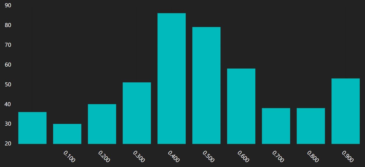
The spread command is used to organize values into a defined number of buckets. These buckets can contain metrics. This is useful for generating histograms from a smoothly varying input field.
{
    $spread: {
        path:"<the statement path to the input values>",
        min:"<the minimum possible value>",
        max:"<the maximum possible value>",
        count:"<the count of buckets to generate>",
    },
},
For instance, a bar chart showing the count of all the scaled scores (which normally run from 0 to 1) would produce a graph with many many bars, each with a single value. Something like this:

This is not really a histogram. This chart shows you the relative count of values, not the distribution of values. Sorting by the x label would improve things, but you would still be selecting the top N unique scores, and plotting their frequency. To get an accurate view of the data, you'd have to make sure you asked for enough bars that there was a bar for every unique value in the data set. On a smooth scale, this could be unlimited. Likewise, the score .8000001 and .8 would be counted separately, with a bar for each! A "$frequentValues" is not a good way visualize the distribution over a smooth input field.
{
    process:
    [
        {
            $spread: {
                path: "result.score.scaled",
                max:1.00,
                min:0,
                count:30
            },
        },
        {
            $barChart:{}
        }
    ],
}
The above VQL query will render a 10 bar histogram over the range 0,1 for the score.
A few notes:
The paths command groups statements into lists by some unique value, and computes a few special metrics over the list. It's raw output can be considered as sessions and rendered on a Gantt chart, or the path can be examined using additional logic. The $paths command supports a special $first and $last metric, as well as the normal metrics. It also computes the duration and first and last step in the path for convenience. It sorts statements by timestamp, so path order is maintained.
{
    $paths: {
        stepValuePath:"<which value from the statement is appended to the path list? default: 'object.id'>",
        sessionPath:"<what value marks statements as belonging to each path? default: 'context.registration'>",
    },
},
Because xAPI has a rather flexible representation of session, you must tell the $paths command what path in a statement contains a unique value for each session. While it's possible for an actor to vary across a session, we expect that each statement grouped by the unique values of sessionPath has the same actor. Also, since it's possible for a session to span multiple object.id values, we don't default to this. You'll need to consider your data representation before using this feature.
In general, we assume that the object.id is the "value" of each step in a path. You can override this to be any path in the statement.
{
    $paths: {
        stepValuePath:"result.score.scaled",
        sessionPath:"actor.id",
    },
},
The above configuration of $paths will build an ordered list of each score on any activity by actor.
{
    $paths: {
        stepValuePath:"context.extensions['http://example.com/module'].id",
        sessionPath:"context.contextActivities.grouping.id",
    },
},
The above configuration of $paths will build an ordered list of each module.id from the context extensions based on a session ID stored in the grouping context activities (which is typical of SCORM profile xAPI data.)
The $paths stage supports 2 special case metrics, $first and $last. When statements are pushed onto a list to generate he path, these metrics will pull either the first or last value seen for a given path.
{
    $paths: {
        stepValuePath:"object.id",
        sessionPath:"context.registration",
        metrics:{
            success:{
                $last:"result.complete"
            },
            actor:{
                $last:"actor.id"
            }
        }
    },
},
The above configuration will pull paths across objects by registration, and find the completion status of the final item. We'll also pull the actor name. Since we assume that a registration is unique to an actor, either the first or the last actor.id will tell us the actor of the whole session.
output
[
    {
        _id: "3a336b33-d520-4602-a674-767225a7025f",
        path: [
            "http://example.com/mini-game",
            ...
        ],
        duration: 1038555,
        first: "http://example.com/mini-game",
        last: "http://example.com/mini-game",
        length: 8,
        start: "2019-06-14T08:51:13.018Z",
        end: "2019-06-14T09:08:31.573Z"
    },
    ...
The above document shows the output from a $path command with no metrics. The fields are
The $ratio command provides a shorthand for computing relative number of statements matching 2 queries
{
    $ratio:{
        of: "<filter>",
        over: "<filter>"
    }
},
This command is a shortcut to run 2 queries in parallel and compute their relative counts. Note that these sub filters are expanded into sub $queries, and therefore follow the filter inheritance rules. Both the 'of' and 'over' properties should be filters exactly as described in the filter section. $ratio does not support metrics.
{
    $ratio:{
        of: {
            "verb.id": "http://adlnet.gov/expapi/verbs/scored",
            "result.score.scaled":{ $gt:.7}
        },
        over: {
            "verb.id": "http://adlnet.gov/expapi/verbs/launched"
        },
    }
},
The above example computes the ratio of statements where a verb matches "scored" and the score is greater than .7 over the number of total launches.
output
[
    {
        ratio: 0.2727272727272727
    }
]
$Ratio will output a single document, with one key. This key is always "ratio", and is the result of the count of statements matching the first filter to those matching the second.
Count the number of document in the stream, or the number of statements that match the filter. The only configuration is what the name of the output value will be.
{
    $count:"<outputKey>"
},
output
[
    {
        outputKey: 264 //The number of matches
    }
]
When this command is the first command in the processing pipeline, it matches against statements themselves. This can be done very efficiently. When it is not the first, it counts the number of documents in the stream.
This stage is used to compute an expression. It destroys the input stream, meaning that its only use is if the expression is known at plan time. The intention is to allow the use of $inlineSubQuery to form the expression. The stage always outputs an array containing a single document
{
    {
        $expression:{
            $subtract:[1,3]
        }
    },
},
The above stage results in the following output document array.
[
    {
        "value": -2
    }
]
This of course is of limited utility. Use this stage with $inlineSubQuery. Here's a great example
{
    {
        $expression:{
            $subtract:[ {
                $inlineSubQuery:{
                    filter:{
                        "verb.id":"...passed"
                    },
                    process:[
                       {$count:"count"}
                    ],
                    select:{
                        mode:"one",
                        path:"$[0].count"
                    }
                }
            } ,{
                $inlineSubQuery:{
                    filter:{
                        "verb.id":"...failed"
                    },
                    process:[
                       {$count:"count"}
                    ],
                    select:{
                        mode:"one",
                        path:"$[0].count"
                    }
                }
            } ]
        }
    },
},
This finds 2 counts of different verbs, and subtracts one from the other. Note the query plan:
{
            "type": "ExpressionStage",
            "args": {
                "expr": {
                    "$subtract": [
                        1514,
                        364
                    ]
                },
                "lrs": "102d1251-0d5c-491e-b87b-250061a9d7f8"
            }
        }
The $inlineSubQuery turns this into a static computation.
These commands can be used to find the min, max, sum average or standard deviation of values. Each takes only a path setting, which identifies the location in the statement or document to process.
{
    $min: {
        path: "<A statement path>"
    }
},
output
[
    {
        value: 264
    }
]
When these commands are the first command in the processing pipeline, they match against statements themselves. This can be done very efficiently. When not the first, they compute over documents in the stream.
While not obviously powerful on their own, these commands can be used in combination with a filter to ask "What is the average score on this exam", or "Of all their attempts, what is the longest a student ever spent in the module?"
This command returns information about the structure of data. It takes a single parameter 'path', and returns an array representing the possible child document keys and their data types.
{
    $keys:{
        path:"result"
    }
},
output
[
    {
        _id: "duration",
        type: "string"
    },
    {
        _id: "extensions",
        type: "object"
    },
    {
        _id: "score",
        type: "object"
    },
    {
        _id: "success",
        type: "boolean"
    }
]
Use this command to reflect on the structure of unknown data, especially in extensions, where the xAPI schema provides no information.
This command is used to map some agent, activity or verb to its "canonical" representation. This is very useful if your dataset does not include the pretty name or description in every verb. You can join to that data with the command, and only send a simple verb.id with most statements. Note: you should use this command as late in your process as you can, because it requires exiting the database and continuing processing in JavaScript. In some cases, this can have a massive performance penalty, so use this only right before a rendering command.
{
    $toCanonicalDisplay:{
        path:"<a JSON path to an identifier. Default:'_id'>",
        outkey:"<the property name at which to append the canonical data. Default:'canonical'>",
        mode:"either 'any','activity','agent', or 'verb'"
    }
},
In many cases, using only the defaults will accomplish the goal. You can increase efficiently by letting the system know if you expect the value to represent an agent, activity or verb. By default, it will query all three tables and return the first match.
Given an input stream of documents like
[
    {
        _id:"mailto:[email protected]",
        count: 264,
    },
    ...
]
{
    $toCanonicalDisplay:{}
}
The above command will result in a stream of documents like
{
    [
    {
        _id: "mailto:[email protected]",
        count: 264,
        canonical: {
            _id: "5d08fc24aa70bd4ba10d2970",
            id: "mailto:[email protected]",
            account_homepage: null,
            account_name: null,
            count: 264,
            created: "2019-06-18T14:58:44.448Z",
            display: "Amelia Duval",
            isActor: true,
            mbox: "mailto:[email protected]",
            mbox_sha1sum: null,
            name: "Amelia Duval",
            updated: "2019-06-18T14:59:17.104Z"
        }
    },
    ...
}
$toCanonicalDisplay can also map sub arrays. When path contains a *, we'll compute the value for each object in an embedded array.
[
    {
        "_id": "Amelia Duval",
        "objects": [
            {
                "_id": "http://example.com/mini-game",
                "count": 84
            },
            {
                "_id": "http://example.com/simple-example",
                "count": 80
            },
            ...
        ]
    },
    ...
]
When give the above document stream
{
    $toCanonicalDisplay: {
        path: "objects[*]._id",
    }
},
The above command will produce the following output.
[
    {
        _id: "Amelia Duval",
        objects: [
            {
                _id: "http://example.com/mini-game",
                count: 84,
                canonical: {
                   ...
                }
            },
            {
                _id: "http://example.com/simple-example",
                count: 80,
                canonical: {
                   ...
                }
            },
            {
                _id: "http://example.com/standard-scenario",
                count: 52,
                canonical: {
                    ...
                }
            },
            {
                _id: "http://example.com/cdiff-scenario",
                count: 48,
                canonical: {
                   ...
                }
            }
        ]
    },
    ...
]
Each sub document in the embedded 'objects' array has had its' '_id' mapped to 'canonical'. This is particularly useful when using a renderer that understands embedded arrays.
This stage works very much like the $toCanonicalDisplay stage, but is used to map a response ID to the response display text from the canonical table for CMI type interactions
{
    $toCanonicalResponse:{
        path:"<a JSON path to an identifier. Default:'_id'>",
        outkey:"<the property name at which to append the canonical data. Default:'canonical'>",
        objectId: "<a hardcoded single activity ID that is used to look up from the canonical tables>",
        objectIdPath: "<a json path expression used to identify the proper activity per input document (for instance if the incoming document stream has responses from multiple different activities)>"
    }
}
Add a field to each document. This field can be computed using expression commands. We borrow this directly from MongoDB, so read the documentation here.
Restructure the existing document by computing new fields from old ones. We borrow this directly from MongoDB, so read the documentation here.
VQL includes a few basic commands for iteration, parallel processing, and sub queries. Additionally, there are some special symbols that dictate how data is passed around within complex queries.
There is a special processing stage which can represent a sub query. These sub queries can be used to "go back to the database" to compute additional values. Sub queries follow a set of rules for deciding how they interact with a parent query.
{
    filter:null,
    process:
    [
        {
            $query:{
                filter: {
                    "result.score.scaled":1
                }
            }
        }
    ]
}
The above query will simply return a list of statements where "result.score.scaled" is 1.
{
    filter:null,
    process:
    [
        {
            $query:{
                filter: {
                    "result.score.scaled":1
                }
            }
        },
        {
            $query:{
                filter: {
                    "result.score.scaled":0
                }
            }
        }
    ]
}
In the example above, the second sub query destroys the results of the first. This is a significant waste of compute resources, and should be avoided.
{
    filter:{
        "actor.id":"mailto:[email protected]"
    },
    process:
    [
        {
            $query:{
                filter: {
                    "result.score.scaled":1
                }
            }
        },
    ]
}
In the above example, the subquery will find statements where the actor.id is "mailto:[email protected]" AND the scaled score is 1. This is because the subquery inherits the parent filters
{
    filter:{
        "actor.id":"mailto:[email protected]"
    },
    process:
    [
        {
            $query:{
                filter: {
                    $inherit:false,
                    "result.score.scaled":1
                }
            }
        },
    ]
}
In the above example, the subquery will find statements where scaled score is 1, regardless of the parent query actor.id filter. This is because $inherit is false
{
    filter:{
        "actor.id":"mailto:[email protected]"
    },
    process:
    [
        {
            $count:"count"
        },
        {
            $query:{
                filter: {
                    "result.score.scaled":1
                }
            }
        },
    ]
}
Similarly, the value of $count above is lost. What then is the purpose of a subquery at all? Read on.
The parallel command allows you to run multiple queries in parallel. The results of each stage will be an element in the output array, meaning that you'll end up with nested arrays.
{
    filter: {
        "actor.id": "mailto:[email protected]"
    },
    process:
    [
        {
            $parallel:{
                stages:[
                    {
                        $query:{
                            filter:{},
                            process:[
                                {
                                    $min: {
                                        path: "result.score.scaled",
                                    },
                                },
                            ]
                        }
                    },
                    {
                        $query:{
                            filter:{},
                            process:[
                                {
                                    $max: {
                                        path: "result.score.scaled",
                                    },
                                },
                            ]
                        }
                    }
                ]
            }
        }
    ],
}
The above query will result in an array of 2 data sets. Since each stage in the $parallel is a query, it outputs an array. Because the $min and $max stages always output one document, the results will be
[
    [
        {
            "value": 0.009999999776482582
        }
    ],
    [
        {
            "value": 1
        }
    ]
]
Note that the sub queries inherit the parent filters. In almost all circumstances, the child stages should be queries.
{
    filter: {
        "actor.id": "mailto:[email protected]"
    },
    process:
    [
        {
            $parallel:{
                stages:[
                    {
                        $min: {
                            path: "result.score.scaled",
                        },
                    },
                    {
                        $max: {
                            path: "result.score.scaled",
                        },
                    },
                ]
            }
        }
    ],
}
The above structure is not currently supported. The min and max stage will compute over the whole data set, because they are not "query consuming" commands, and are nested in such a way that the planner cannot plan their filters. The planner will instead select 1000 results that match the filter, move them into JavaScript, and compute the min and max there. This can be accurate, but you'll never know if there was additional data to consider or not. This construction may be supported in the future.
Note: There are several patterns that cause the planner to retrieve data from the database and continue processing the query in JavaScript. When this happens, the initial dataset is confined to some maximum number of results, 1000 currently. In general, query patterns that compute in this mode are inefficient and can be inaccurate. You should strive to form queries that can be computed mostly in the database. Check the output of $explain for query execution data.
In the above example, the result of a query was a set of nested arrays. $mergeArrays will concatenate these arrays and output a single array.
{

    filter: {
    process:
    [
        {
            $parallel:{
                stages:[
                   ...
                ]
            }
        },
        {
            $mergeArrays:{}
        }
    ],
}
Will produce
[
    {
        "value": 0
    },
    {
        "value": 1
    }
]
rather than
[
    [
        {
            "value": 0
        }
    ],
    [
        {
            "value": 1
        }
    ]
]
This can make continued processing much simpler. For instance, you might find the maximum score for several students and then average those scores.
{

    filter: {
    process:
    [
        {
            $parallel:{
                stages:[
                   ...
                ]
            }
        },
        {
            $mergeArrays:{}
        },
        {
            $avg:{
                path:"$value"
            }
        }
    ],
}
This command will replace the result set with a lengthy report on what the query engine actually did. Because there can be different ways to describe the same logic, you may wish to compare speeds, or debug your logic. This command lets you see stage timings and the results at each step in the computation. Explain current accepts no settings. Any value will work, though in the future we may opt to select certain types of data in the settings.
{
    $explain:true
}
VQL uses special JSON objects to allow a variety of functionality.
$inlineSubQuery is a plan time subquery. It can be used to make a query and feed the results into the the formation of a higher level sub query. This allows more expressive syntax than using a combination of a $query stage and they $input keyword, although the results are similar.
{
    filter: {
        "actor.id": {$in:{
            $inlineSubQuery:{
                select:{
                    path:"$[*]._id",
                    mode:"all"
                },
                filter:{

                },
                process:[
                    {
                        $frequentValues:{
                            path:"actor.id"
                        }
                    },

                ]
            }
        }}
    },
    process:
    [

    ]
}
The above example finds the 10 most frequent actors, and gets statements by those actors (without processing them). Note that the query plan actually shows the computed result of the subquery in the plan. The filter for the actual query shows this:
    "filter": {
        "actor.id": {
            "$in": [
                "6e4c2cd96ae7366434fcde2990b9c4aecd194235",
                "237a069230bd63a33a199308c7051ea8b3782fb0",
                "aec226e629317cd1dff60fda5913450ffba304ee",
                "8811f8c8fde39e96233499dd99a2dffa42bf9106",
                "a986c5de80ec830429649599d5547fc574c6e39e",
                "e979eabe1cee325ec09e0cc98b2c93c18045726a",
                "41595cc08504104e89e35c61ba58ed00b3a038c8",
                "80cd17a320ecb1df3fc7f475ee83e2f88dc76e5d",
                "fedf814142928dbf6047c4ece8058fa9990b17bc",
                "e36cfe9d632c8fa2cc499445d1d2420f0f674269"
            ]
        }
    },
Where the $in query operator has an array - this array is the output from the $inlineSubQuery. Note the select field in the example above. It is frequently necessary to extract some particular value from the subquery result.
So, in order to find statements by the single most frequent agent, you would form the $inlineSubQuery as:
{
    filter: {
        "actor.id":{
            $inlineSubQuery:{
                select:{
                    path:"$[0]._id",
                    mode:"one"
                },
                ...
            }
        }
    },
    process:
    [

    ]
}
The computed filter for the query then becomes
   "filter": {
        "actor.id": "6e4c2cd96ae7366434fcde2990b9c4aecd194235"
    },
    ...
$input allows you to reference the values that flow into a query, if that query is not the first in a process. The $input keyword is evaluated at query planning time - which for a subquery command comes when that subquery is executed. This means that you can make a query that depends on the values of a previous query!
{
    filter:{},
    process:
    [
        {
            $query:{
                filter: {},
                process:[
                    {
                        $avg:{
                            path:"result.score.scaled"
                        }
                    }
                ]
            }
        },
        {
            $query:{
                filter: {
                    "result.score.scaled":{
                        $gt:{
                            $input:{
                                path:"$[0].value"
                            }
                        }
                    }
                },
                process:[
                    {
                        $frequentValues:{
                            path:"actor.id"
                        }
                    }
                ]
            }
        },
    ]
}
Consider the above example. It uses two subqueries in sequence, feeding the results of one process into the query of another. The first query, run alone, returns a data set like this:
[
    {
        "value": 0.5000182093987425
    }
]
The value is the average score of all statements because the filter is blank. Because $input is resolved at execution time,
$input:{
    path:"$[0].value"
}
becomes
0.5000182093987425
Therefor the filter for the second query becomes
"result.score.scaled":{
    $gt:0.5000182093987425
}
Since there is no query at the top level, the second subquery will filter the full data set. This can be summed up as
"Find the average, and then find the people who most frequently score higher."
{
    $input:{
        path:"<a JSON path>",
        mode:"<'all' or 'one'>"
    }
}
the $each command makes it simpler to execute the same process in parallel for multiple filters. When $each is found in a query filter, that queries process is automatically "unwound" to a set of $parallel $queries for $each different value. For instance
{
    filter:{
        $each:[
            {
                "actor.id":"[email protected]",
                "activity.id":"https://www.example.com/module"
            },
            {
                "actor.id":"[email protected]",
                "activity.id":"https://www.example.com/module"
            },
            {
                "actor.id":"[email protected]",
                "activity.id":"https://www.example.com/module"
            }
        ]
    },
    process:[
        {
            $frequentValues:{
                path:"result.response"
            }
        }
    ]
}
will internally expand into
{

    filter:{

    },
    process:[
        {
            $parallel:{
                stages:[
                    {
                        $query:{
                            filter:{
                                "actor.id":"[email protected]",
                                "activity.id":"https://www.example.com/module"
                            },
                            process:[
                                 {
                                    $frequentValues:{
                                        path:"result.response"
                                    }
                                }
                            ]
                        }
                    },
                    {
                        $query:{
                            filter:{
                                "actor.id":"[email protected]",
                                "activity.id":"https://www.example.com/module"
                            },
                            process:[
                                 {
                                    $frequentValues:{
                                        path:"result.response"
                                    }
                                }
                            ]
                        }
                    },
                    ...
                ]
            }
        }
    ]
}
In fact, the same logic can be expressed even more concisely by inverting the location of the $each
{
    filter:{
        "actor.id":{
            $each:["[email protected]","[email protected]","[email protected]"],
        },
        "activity.id":"https://www.example.com/module"
    },
    process:[
        {
            $frequentValues:{
                path:"result.response"
            }
        }
    ]
}
The above example shows how you can use $each to process a list of IDs. In fact, you can merge $each with $input and $query to find some list, and then repeat a process for each value in that list. For instance:
{
    filter:null,
    process:[
        {
            $query: {
                filter:{
                    "activity.id":"https://www.example.com/module"
                },
                process:[
                    {
                        $frequentValues:{
                            path:"actor.id"
                        }
                    }
                ]
            }
        },
        {
            $query: {
                filter:{
                    "actor.id":{
                        $each:{
                            $input:{
                                path:"$[*]._id",
                                mode: "all"
                            }
                        }
                    },
                    "activity.id":"https://www.example.com/module"
                },
                process:[
                    {
                        $frequentValues:{
                            path:"result.response"
                        }
                    }
                ]
            }
        }
    ]
}
The above example finds the most frequent actors on a module, and then, for each of them, finds their most frequent responses. NOTE: this particular example could also be computed with a $frequentValues and a sub $frequentValues metric.
There are a variety of times when you need to know some additional value to build the query, but will only know that value after the query has been submitted. The $context keyword is used to replace part of the query with such a value before the query executes. The parameters are the same as $input, and the logic works the same way - you select one or all results of a JSON path and replace the $context call with those values. The path is evaluated against the "context object", which varies with different applications of VQL.
{
    $context:{
        path:"<a JSON path>",
        mode:"<'all' or 'one'>"
    }
}
$context will always include the current filter and process of the current query. When executing a sub query, a new "context object" is generated, and the context of the parent query is available as "$parent.xxx". So, in a sub query, to access the top level filter, you can written
{
    $context:{
        path:"$parent.filter['actor.id']"
    }
}
When using the automatic $parallel generate by each, you can get the value of the currently executing branch to use for a title in a rendering command.
{
    filter: null,
    process: [
        {
            $query: {

                filter: {
                    $each: [
                        { "actor.id": "mailto:[email protected]" },
                        { "actor.id": "mailto:[email protected]" },
                        { "actor.id": "mailto:[email protected]" },
                    ]
                },
                process: [
                    {
                        $frequentValues: {
                            path: "object.id",
                        },
                    },
                    {
                        $barChart: {
                            categoryPath: "canonical.display",
                            seriesTitle: {
                                $context: {
                                    path: "$.filter['actor.id']"
                                }
                            }
                        }
                    }
                ]
            }
        },

    ]
}
The above example uses $context to give a series title to each bar chart that is generate by $each.
$defThe $def command allows you to extract a bit of VQL and reuse it in multiple places in a query. The values that are used to populate a $def are stored in the top level query object, or passed into the $def command when it's used.
{
    filter:null,
    process:[
        {
            $expression:{
                 min: {$def:"min"},
                 max: {$def:"max"},
            }
        }
    ],
     defs:{
        min:0,
        max:100
    }
}
Results in the result:
[
    {
        "value": {
            "min": 0,
            "max": 100
        }
    }
]
Of course, this could be much more interesting!
{
    {
    filter:null,
    process:[
        {
            $expression:{
                 min: {$def:"min"},
                 max: {$def:"max"},
            }
        }
    ],
     defs:{
        min:{
            $inlineSubQuery:{
                filter:null,
                process:[
                    {$max:{path:"result.score.scaled"}}
                ],
                select:{
                    mode:"one",
                    path:"$[0].value"
                }}
        },
        max:{
            $inlineSubQuery:{
                filter:null,
                process:[
                    {$min:{path:"result.score.scaled"}}
                ],
                select:{
                    mode:"one",
                    path:"$[0].value"
                }}
        }
    }
}
The above query actually computes something, by using 2 $inlineSubQuery commands. However, we've not really saved much buy using the defs, since each def is used once and only once. This does not decrease the amount of code. We can simplify further by parameterizing the defs like so.
{
    filter:null,
    process:[
        {
            $expression:{
                 min: {$def:{path:"minOrMax",defs:{param:{$min:{$def:"score"}}}}},
                 max: {$def:{path:"minOrMax",defs:{param:{$max:{$def:"score"}}}}},
            }
        }
    ],
     defs:{
        score:{path:"result.score.scaled"},
        minOrMax:{
            $inlineSubQuery:{
                filter:null,
                process:[
                    {$def:"param"}
                ],
                select:{
                    mode:"one",
                    path:"$[0].value"
                }}
        },
    }
}
Here, the def minOrMax uses other defs inside its definition. From where are these filled? From the values in the defs field of the $def command. This is essentially the same idea as a function call. We call the def that defines a subquery and pass new defs to resolve the full inlineSubQuery. Just to make things more amazing, the value we pass into minOrMax references the score definition. You can sort of imaging score like a function call that takes no parameters and returns a literal string.
One major goal of VQL is to harmonize visualization and data processing. To achieve that goal, VQL includes commands that will translate data into a graph configuration object. This object is then fed to the renderer in the client to produce the graph. In Veracity Learning, graphs are rendered with Amcharts, and therefore the rendering commands output an Amcharts compatible graph description.
Rendering commands are simply another command in a process. They will render the incoming document stream according to their own settings. Some rendering commands will modify the incoming stream to make it compatible with the renderer.
Several rendering commands support "split rendering", where each document in the stream contains an array field. When appropriately configured, the renderer will "split" the widget - so that a bar chart becomes a stacked bar, a pie chart becomes a sunburst, or a line chart has multiple lines.
The $barChart command generates one bar for each incoming document in the stream. The height of the bar (the 'value') is one of the properties in the document. $barChart supports split series rendering. The $barChart defaults are aligned with the $frequentValues stage, so you can render a basic $frequentValues with no configuration.
{
    $barChart:{
        categoryPath: '_id',
        valuePath : 'count',
        stackCategory : '_id',
        stackTitle : '_id',
        titlePath : '_id',
        seriesTitle : "a string",
    }
}
{
    filter: {
    },
    process:
    [
        {
            $frequentValues: {
                path: 'actor.id',
            },
        },
        {
            $barChart: {}
        }
    ],
}
Because the defaults are aligned, you can render a $frequentValues without any configuration. The above query generates the following render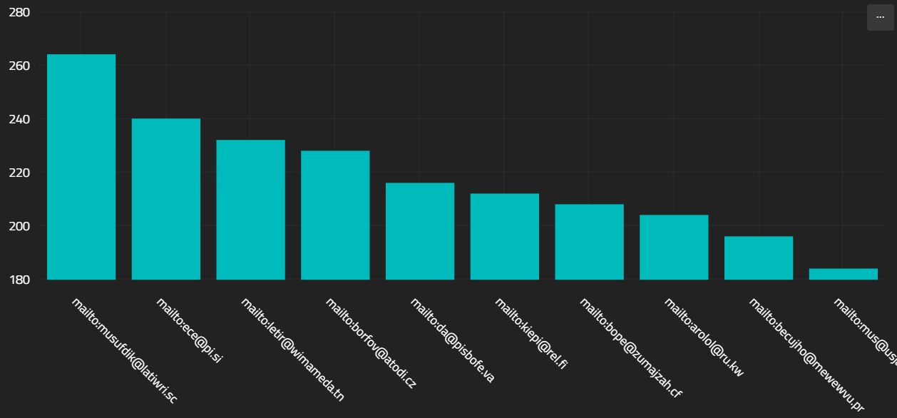
Here,you can see that the _id field became the bar title, and the "count" field became the bar height.
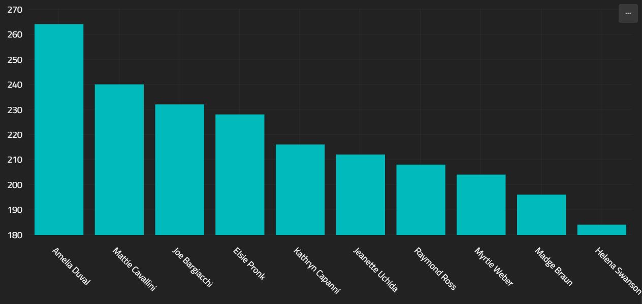
{
    filter: {},
    process:
    [
        {
            $frequentValues: {
                path: 'actor.id',
            },
        },
        {
            $toCanonicalDisplay:{}
        },
        {
            $barChart: {
                categoryPath:"canonical.display"
            }
        }
    ],
}
Above, the $toCanonicalDisplay command adds a property to each document - "canonical.display". The barChart is going to use this, rather than the "_id" field to label the bars.
{
    filter: {
    },
    process:
    [
        {
            $frequentValues: {
                path: 'actor.id',
                metrics:{
                    avgScore: { $avg: "result.score.scaled" }
                }
            },
        },
        {
            $barChart: {
                valuePath:"avgScore"
            }
        }
    ],
}
Above, you can see a query that computes a metric. Because the metric will add a property called "avgScore" to each document in the stream, the $barchart stage is configured to make the height of the bar the value of the "avgScore" field.
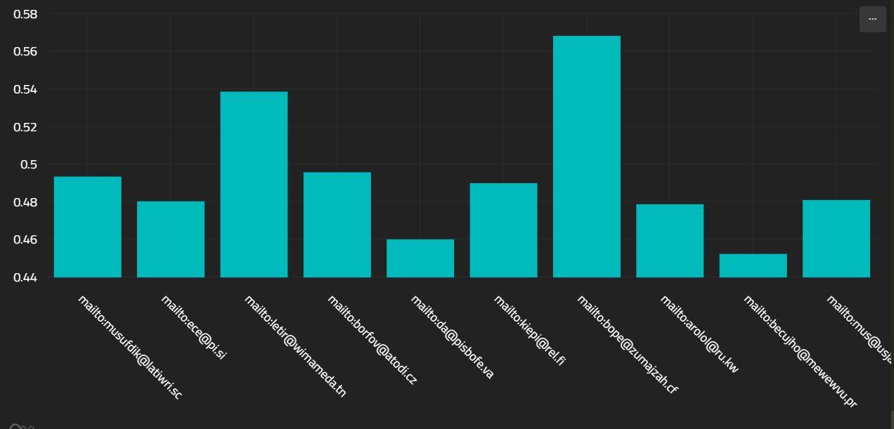
Note: The above query computes the average score of the most frequent 10 actors, not the 10 top average scores. See $frequentValues.
The $barChart (and $pieChart and $serialChart) commands can detect a split series render. To enable this, you must first have a document stream that contains a property that is itself a list of objects. This is commonly achieved with a $frequentValues that has a metric of the special type $frequentValues or $timeSeries. When the data contains these subseries, you can use a JSON path to select into this subseries for the valuePath and categoryPath. As usual, the defaults are aligned to minimize verbosity of the most common cases.
{
    filter: {},
    process:
    [
        {
            $frequentValues: {
                path: 'actor.id',
                metrics:{
                    objects:{
                        $frequentValues: { path: "object.id" }
                    }
                }
            },
        },
        {
            $barChart: {
                valuePath:"objects[*].count",
                categoryPath:"objects[*]._id"
            }
        }
    ],
}
Notice how the categoryPath and valuePath above use array notation to select into the subseries called "objects". The '*' lets the renderer know that you wish to split the series. Note also that the categoryPath an valuePath both select the same subseries. This is mandatory.
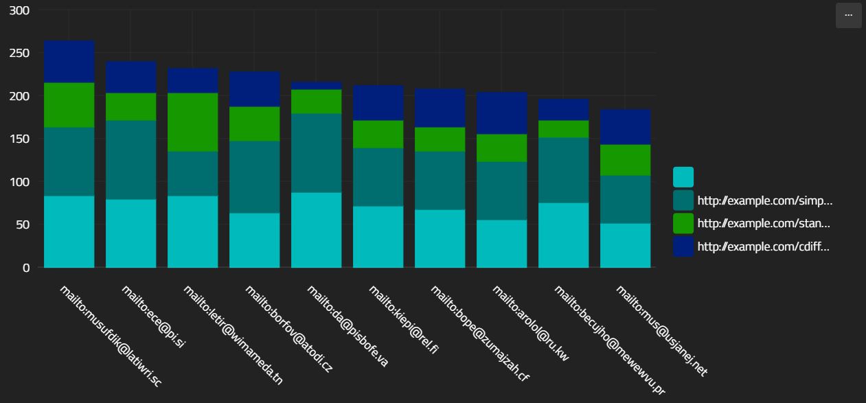
One thing to note - each stack of bars is titled with the _id of the parent object. You can override this by using the "stackCategory" property. Consider:
{
    filter: {},
    process:
    [
        {
            $frequentValues: {
                path: 'actor.id',
                metrics:{
                    objects:{
                        $frequentValues: { path: "object.id" }
                    }
                }
            },
        },
        {
            $toCanonicalDisplay:{}
        },
        {
            $barChart: {
                valuePath:"objects[*].count",
                categoryPath:"objects[*]._id",
                stackCategory:"canonical.display"
            }
        }
    ],
}
Because the categoryPath is used by the split series features, you use "stackCategory" to let the renderer know how to title the stacks.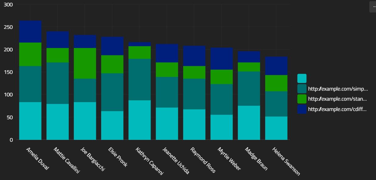
Recall that $toCanonicalDisplay can also map subseries. We'll leave as an exercise to the reader to figure how to make the side legend verb IDs into verb display titles.
In general, you can use the categoryPath or stackCategory values to organize the stacks or bars. It is possible that 2 bars might have different identities, but you wish to display the same title.Imagine 2 actors with the same name. Because they are distinct identities, they should have 2 bars, but both bars would have the same title. In this case, use categoryPath to tell the renderer what makes a document unique, and titlePath to select the title that will be displayed.
The $pieChart is almost identical logically to the $barChart. It generates one slice for document in the stream. It also supports a split series.

When rendering a split series, the $pieChart will generate a visualization called a "sunburst" diagram.
The $serialChart is for rendering time series. It works in much the same way, with slightly different parameters. The defaults are aligned with the $timeSeries stage, so you can produce an "Activity over time" graph for a filter very easily
{
    filter: {
    },
    process:
    [
        {
            $timeSeries: {},
        },
        {
            $serialChart: {}
        },
    ],
}
The above will create a simple line chart of all traffic over time. This is because the default valuePath is "count", which is always included in a $timeSeries. One major difference - when a $serialChart has only a single line, there is no "title" for that line.
{
    "filter": {},
    "process": [
        {
            "$frequentValues": {
                "path": "actor.id",
                "metrics": {
                    "objects": {
                        "$timeSeries": {
                            "path": "timestamp"
                        }
                    }
                }
            }
        },
        {
            "$serialChart": {
                "categoryPath": "objects[*]._id",
                "valuePath": "objects[*].count",
            }
        }
    ]
}
Because a $frequentValues can have a special type of metric which is a $timeSeries, you can configure the renderer to produce a multi line chart.
Similar to "stackCategory" and "stackTitle", "lineCategory" and "lineTitle" can be used to name sub series.
{
    filter: {},
    process: [
        {
            $frequentValues: {
                path: "actor.id",
                metrics: {
                    objects: {
                        $timeSeries: {
                            path: "timestamp"
                        }
                    }
                }
            }
        },
        {
            $toCanonicalDisplay:{}
        },
        {
            $serialChart: {
                categoryPath: "objects[*]._id",
                valuePath: "objects[*].count",
                lineCategory:"canonical.display"
            }
        }
    ]
}
Notice above that the lineCategory selects the value from the root object. This is because there is no use in naming each point on a line, only the whole line itself. This differs somewhat from a split bar or pie, where each block or slice can be named.
A $notice render is a large, centered bit of text with an icon, and a subtext section below. A $notice render only shows data from the 0th document in the incoming stream.
{
    $notice: {
        subtitle: "Demo Title",
        title: "The subtext goes here",
        icon: "check",
    }
}
The above rendering command produces the below image.
You may notice that this render is not modified by the incoming data at all! Read on...
The $notice and $list renderers use a special format of string to select values to display.
{
    $notice: {
        subtitle: "${value._id} was launched ${value.count} times",
        title: "${value.canonical.display}",
        icon: "check",
        valuePath: "$",
    }
}
the above render will template in the values from the 0th document in the stream. You can use logic upstream from the renderer along with this feature to customize the icons and colors as well.
{

"filter": {},
    title: "Top Agents",
        "process": [
            {
                $frequentValues: {
                    path: "actor.id",
                    metrics:{
                        avgScore:{
                            $avg:"result.score.scaled"
                        }
                    },
                    limit: 7
                }
            },
            {
                $skip:1
            },
            {
                $toCanonicalDisplay: {}
            },
            {
                $project:{
                    avgScore:"$avgScore",
                    count:"$count",
                    canonical:"$canonical",
                    icon:{
                        $switch:{
                            branches: [
                              { case: {$gt: [ "$avgScore", 0.49 ]}, then: "check" },
                           ],
                           default: "close"
                        }
                    },
                    color:{
                        $switch:{
                            branches: [
                              { case: {$gt: [ "$avgScore", 0.49 ]}, then: "green" },
                           ],
                           default: "red"
                        }
                    }
                }
            },
            {
                $notice: {
                    subtitle: "${value._id} scored ${value.avgScore}%",
                    title: "${value.canonical.display}",
                    icon: "${value.icon}",
                    valuePath: "$",
                    color:"${value.color}",
                    precision:2
                }
            }

        ]
}
The above example uses to switches as part of a projection to compute values for the icon and color. Then, it uses string interpolation to use those computed values in the renderer.
It's important to note that these values are dynamic. Depending on the data in the statement, you may see either a red X or a green check.
The $list command works identically to the $notice command, except it renderers each document in the incoming stream.
The above render is produced by the exact same query as the notice example above, with the command $notice changed to $list.
A heatChart build a 2D grid of boxes, colored according to a metric. It's intended to work with the $punchCard command, but does not yet match the default document format. Therefor, you'll have to provide a bit of logic before the render. IT can also be used to visualize any list of documents with 2 category axes and one value axis.
{
    $heatChart:{
        categoryPathY:"<Must be a simple property name. Not a full JSON Path>"
        categoryPathX:"<Must be a simple property name. Not a full JSON Path>"
        valuePath:"<Must be a simple property name. Not a full JSON Path>"
    }
}
{
    filter: {},
    process:
    [
        {
            $punchCard:{
                path:"timestamp",
                metrics:{
                    score:{
                        $avg:"result.score.scaled"
                    }
                }
            }
        },
        {
            $unwind:"$hours"
        },
        {
            $project:{
                day: "$day",
                hour:"$hours.hour",
                count:"$hours.count",
                score:"$hours.score",
            }
        },
        {
            $heatChart:{
                categoryPathX:"day",
                categoryPathY:"hour",
                valuePath:"score"
            }
        }

    ]
}
Above, you can see the projection that is required to prepare the data for render.
You can see that the average score is used to plot the color. Dark gray is .38 and bright blue is .64. Min and max values are computed automatically.
The ganttChart renderer displays sessions as bars on a date axis. Its defaults are aligned with the $paths command, so you can render $paths as sessions on the ganttChart without any configuration.
{
    $ganttChart:{
        categoryPath: "<a unique identifier for the "row". All sessions that have the same value appear on the same row. Default: '_id'>"
        startPath: "<the path to a timestamp that opens the session>"
        endPath: "<the path to a timestamp that closes the session>"
    }
},
The ganttChart does not support any additional configuration.
{
    filter: {},
    process: [
        {
            $paths:{
                sessionPath:"context.registration",
            }
        },
        {
            "$ganttChart":{}
        }
    ]
}
The above render creates a row for every different session, because the _id of the each $path is a context.registration, which is unique per session.
This query create a very large chart! You can zoom and scroll with the bars on the top and right.
{
    "filter": {

    },
    "process": [
        {
            "$paths":{
                "sessionPath":"context.registration",
                "metrics":{
                    "actor":{
                        "$last":"actor.id"
                    }
                }
            }
        },
        {
            "$limit":50
        },
        {
            "$ganttChart":{
               categoryPath:"actor"
            }
        }

    ]
}
In the above query, we use a $last special metric to grab the name of the actor in the session. Also, we limit the amount of data just for display. The categoryPath is set to "actor", so now rows use the actor name, and sessions that have the same actor are rendered on thee same row.
VQL includes some special commands for working with paths through content. The most basic is the $paths command, which can generate documents that include ordered lists of steps. These documents can be rendered directly with the $ganttChart, but you might also want to actually visualize the sequences. Doing so requires processing the data with the commands below.
The $pathsToNodes command takes the sequence of steps from $paths and builds a network of nodes with connections. Nodes are connected when a path includes them in sequence. The node weight increase each time the pair is seen.
[
    [A,B,C]
    [B,B,C]
    [B,C,B,C]
]
Consider the above paths. The network of links will be:
A to B = 1
B to C = 4
B to B = 1
C to B = 1
Thus, node A will have 1 outgoing link (to B), node B will have 5 (4 to C and 1 to B) and C will have 1 (to B). In a real world context, these values A,B and C might be lesson identifers. Such a graph of nodes allows us to ask questions like "What lesson do students most frequently take after Earth Science?". When combined with subqueries and filters , you can ask "What lesson do high achieving students most frequently take after Earth Science versus their low achieving peers?"
 {
    $pathsToNodes:{
        order: "<boolean>",
        nodeIdPath: "a JSON path to an identifer that uniquely identifies the node",
        nodeTitlePath: "a JSON path to an identifer that uniquely identifies the node";
    }
},
The defaults are configured to match the output of $paths. Node that the nodeIdPath and nodeTitlePath both operate over the values of the $.path array in each incoming document. By default, these documents are simple strings, and so nodeIdPath and nodeTitlePath can be ignored. Order determines whether or not nodes at different positions in the path should be considered unique. The above example ( with A,B and C) treats order as false. If order were true, then there would be 1 A node, 3 B nodes and 3 C nodes. Because A is always the first, there is only one. B can be the first, second or third, so there are three. Likewise, C and be the second, third or fourth, so there are three.
[
    {
        "_id": "46713ed1-60f3-45a2-a45c-eaefbc3ecd5f",
        "path": [
            "http://example.com/simple-example",
            "http://example.com/mini-game"
        ],
        "duration": 891565,
        "first": "http://example.com/simple-example",
        "last": "http://example.com/mini-game",
        "length": 2,
        "start": "2019-06-18T11:58:12.610Z",
        "end": "2019-06-18T12:13:04.175Z",
        "success": null
    },
    {
        "_id": "e58d3c54-74ca-405e-8fae-845f19479c64",
        "path": [
            "http://example.com/simple-example",
            "http://example.com/mini-game",
            "http://example.com/mini-game",
            "http://example.com/simple-example"
        ],
        "duration": 2747275,
        "first": "http://example.com/simple-example",
        "last": "http://example.com/simple-example",
        "length": 4,
        "start": "2019-06-18T11:48:56.360Z",
        "end": "2019-06-18T12:34:43.635Z",
        "success": null
    },
    ..
Consider a $paths command that outputs the above documents. The $pathsToNodes command will out a series of nodes for each object.id in the $.path.
Output
[
    {
        "in": 5,
        "id": "http://example.com/simple-example",
        "count": 9,
        "objectId": "http://example.com/simple-example",
        "title": "http://example.com/simple-example",
        "out": {
            "http://example.com/mini-game": 2,
            "http://example.com/simple-example": 2,
            "http://example.com/standard-scenario": 1
        },
        "step": "0",
        "totalOut": 5
    },
    ...
]
Above is a single node from the document results stream. You can see it's a node identified by "http://example.com/simple-example", with 3 outputs, each to one of the other nodes. 'objectId' identifies the original value of the object on that path that created the node. Note that the outgoing link describe the other node "objectId", not "id". This is because the "nodeIdPath" can overwrite the value of ID. This object also has total in and total out numbers. These can be subtracted to find a falloff rate.
Such a network of nodes can be rendered directly with a $chordChart command.
{
    $chordChart:{
        titlePath: "<a path to a title for display>"
    }
}
$chordChart takes only one parameter, the titlePath. This is used to title the nodes in the legend. You can use projection logic or $toCanonicalDisplay to generate titles other than the IDs.
Note: chordCharts generally only make sense when the 'order' value of the preceding $pathsToNodes is false.
You can use the titlePath parameter along with $toCanonicalDisplay to map the ids to names.
...
{
    $toCanonicalDisplay:{
        path:"id"
    }
},
{
    $chordChart:{
        titlePath:"canonical.display"
    }
}
Note: colors are selected based on the node title. In the above example changing the node titles changed the colors.
A sankeyChart can be used to visualize the flow through a series of steps. Note that the order parameter of the preceding $pathsToNodes MUST be true, or else the graph can have cycles. The renderer cannot visualize graphs with cycles.
{
    $sankeyChart:{
        titlePath:"<a path to a title for display>"
    }
}
The sankeyChart will render falloff as a fading out line.
{
    $toCanonicalDisplay:{
        path:"objectId"
    }
},
{
    $sankeyChart:{
        titlePath:"canonical.display"
    }
}
Note that when you are mapping a node to some value for display, use the objectId. This is because the id field uniquely identifies the node. When order is false, there are several nodes for each objectId, depending on the location in the path. Therefore, those node ids have an additional integer appended.
Note: colors are selected based on the node title. In the above example changing the node titles changed the colors.
Using the above tools, you can visualize paths and flows. However, that's not all! You can do logic over the nodes before rendering, or even use them as inputs to further logic. As an exercise for the reader - how would you find the average score of students that took the standard-scenario first?
Note: colors are selected based on the node title. In the above example changing the node titles changed the colors.
There are several scenarios where you might generate multiple different charts in a single command. Consider
{
    filter:{
        "actor.id":{
            $each:["[email protected]","[email protected]","[email protected]"],
        },
        "activity.id":"https://www.example.com/module"
    },
    process:[
        {
            $frequentValues:{
                path:"result.response"
            }
        },
        {
            $barChart:{}
        }
    ]
}
The above query will generate 3 bar charts in $parallel! See $each for an explanation. Our renderer does not support a query result that is an array of charts - we need to combine them, or call the renderer once for each result. $mergeCharts can merge multiple line charts, multiple bar charts or multiple pie charts into a "multiseries" bar, pie or serial chart. A multiseries pie or bar differs in that bars are not split, but grouped. Note also that the series title will be displayed if there are multiple series.
The above was generated by
{
    filter: null,
    process: [
        {
            $query: {

                filter: {
                    $each: [
                        { "actor.id": "mailto:[email protected]" },
                        { "actor.id": "mailto:[email protected]" },
                        { "actor.id": "mailto:[email protected]" },
                    ]
                },
                process: [
                    {
                        $frequentValues: {
                            path: "object.id",
                        },
                    },
                    {
                        $toCanonicalDisplay: {
                            path: "_id"
                        },
                    },
                    {
                        $barChart: {
                            categoryPath: "canonical.display",
                            seriesTitle: {
                                $context: "$.filter['actor.id']"
                            }
                        }
                    }
                ]
            }
        },
        {
            $mergeCharts: {}
        }
    ]
}
Note how the $mergeCharts stage is the last stage in the outer process. This example also has a nice example of using $context in $each. $mergeCharts takes no parameters, and will error if the charts are not all of the same type.
Because the rendering expressions actually return JSON objects, you can continue to process the document array after the rendering command! This little trick can be use to customize the colors, axis, labels, or any other components of a chart. Veracity uses AmCharts for rendering, so you can reference their JSON specification here to learn about all the things you can change. Heres a few examples below.
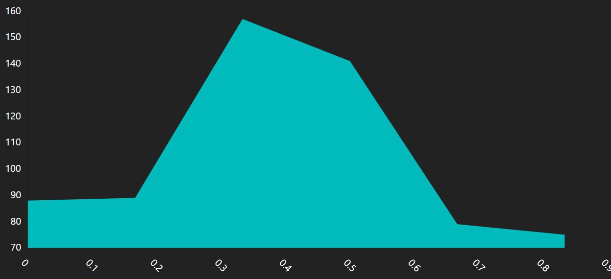
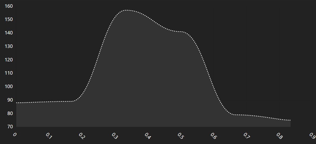
Starting with this render,
    {
        $addFields:{
            "chart.series.0.tensionX":.78,
            "chart.series.0.fill":"#333",
            "chart.series.0.stroke":"#fff",
            "chart.series.0.strokeWidth":2,
            "chart.series.0.strokeDasharray": "3,3",
            "chart.series.0.strokeOpacity": 1,
        }
    }
To color bars in a barChart, you'll need to attach a color value to each entry in the data array, then ask the renderer to use it. This process colors the bars randomly.
        ...
        {
            $addFields:{
                "color": { $arrayElemAt: [ ["red","green","blue"], {$rndInt:{max:4}} ] }
            }
        },
        {
            $barChart:{
                parseDates:false
            }
        },
        {
            $addFields:{
                "chart.series.0.columns.template.propertyFields.fill": "color",
                "chart.series.0.strokeOpacity": 1,

            }
        }
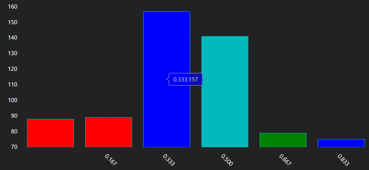
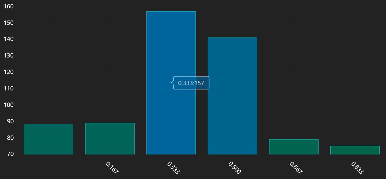
Or you can use some property of the incoming values to compute a color:
{
    process:
    [
        {
            $spread: {
                path: "result.score.scaled",
                max:1.00,
                min:0,
                count:6
            },
        },
        {
            $addFields:{
                "color": { $concat: ["rgb(0,100,", {$toString:"$count"},")"]  }
            }
        },
        {
            $barChart:{
                parseDates:false
            }
        },
        {
            $addFields:{
                "chart.series.0.columns.template.propertyFields.fill": "color",


            }
        }
    ],
}
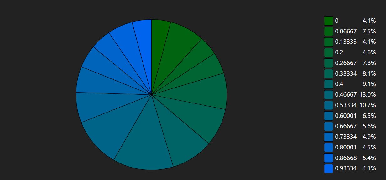
A piechart uses 'slices' instead of 'columns'. Here we compute a gradient, just coloring the slice based on its position in the array.
{
    process:
    [
        {
            $spread: {
                path: "result.score.scaled",
                max:1.00,
                min:0,
                count:15
            },
        },
        {
            $addFields:{
                "color": { $concat: ["rgb(0,100,", {$toString:{$floor:{$multiply:["$_id",255]}}},")"]  }
            }
        },
        {
            $pieChart:{
                parseDates:false
            }
        },
        {
            $addFields:{
                "chart.series.0.slices.template.propertyFields.fill": "color",
                "chart.series.0.strokeOpacity": 1,
                "chart.series.0.slices.template.stroke": "black",

            }
        }
    ],
}
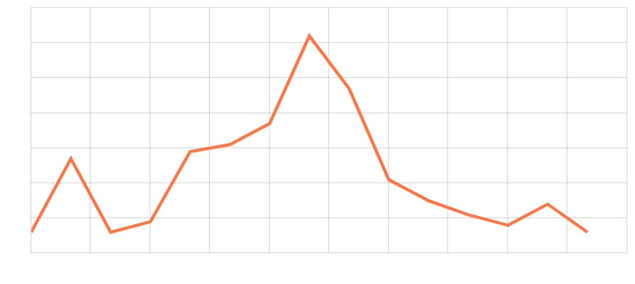
Below is an example that changes the background-color
{
    process:
    [
        {
            $spread: {
                path: "result.score.scaled",
                max:1.00,
                min:0,
                count:15
            },
        },
        {
            $serialChart:{
                parseDates:false
            }
        },
        {
            $addFields:{
                "chart.series.0.fill": "rgba(0,0,0,0)",
                "chart.series.0.fill": "rgba(0,0,0,0)",
                "chart.series.0.strokeOpacity": 1,
                "chart.series.0.strokeWidth": 5,
                "chart.series.0.stroke": "#F74",
                "chart.background.fill":"white",
                "chart.xAxes.0.renderer.grid.strokeOpacity":.2,
                "chart.yAxes.0.renderer.grid.strokeOpacity":.2,
                "chart.xAxes.0.renderer.baseGrid.disabled":true,
            }
        }
    ],
}
You can even radically change the chart by setting the chart and series types
{

    process:
    [
        {
            $spread: {
                path: "result.score.scaled",
                max:1.00,
                min:0.0,
                count:20
            },
        },
        {
            $serialChart:{
                parseDates:false
            }
        },
        {
            $addFields:{
                "chart.series.0.fill": "#8F9",
                "chart.series.0.strokeOpacity": 1,
                "chart.series.0.strokeWidth": 5,
                "chart.series.0.stroke": "#6F4",
                "chart.background.fill":"white",
                "chart.xAxes.0.renderer.grid.strokeOpacity":.2,
                "chart.yAxes.0.renderer.grid.strokeOpacity":.2,
                "chart.yAxes.0.renderer.grid.strokeWidth":2,
                "chart.xAxes.0.renderer.baseGrid.disabled":true,
                "chart.type": "RadarChart",
                "chart.series.0.type":"RadarSeries"
            }
        }
    ],
}
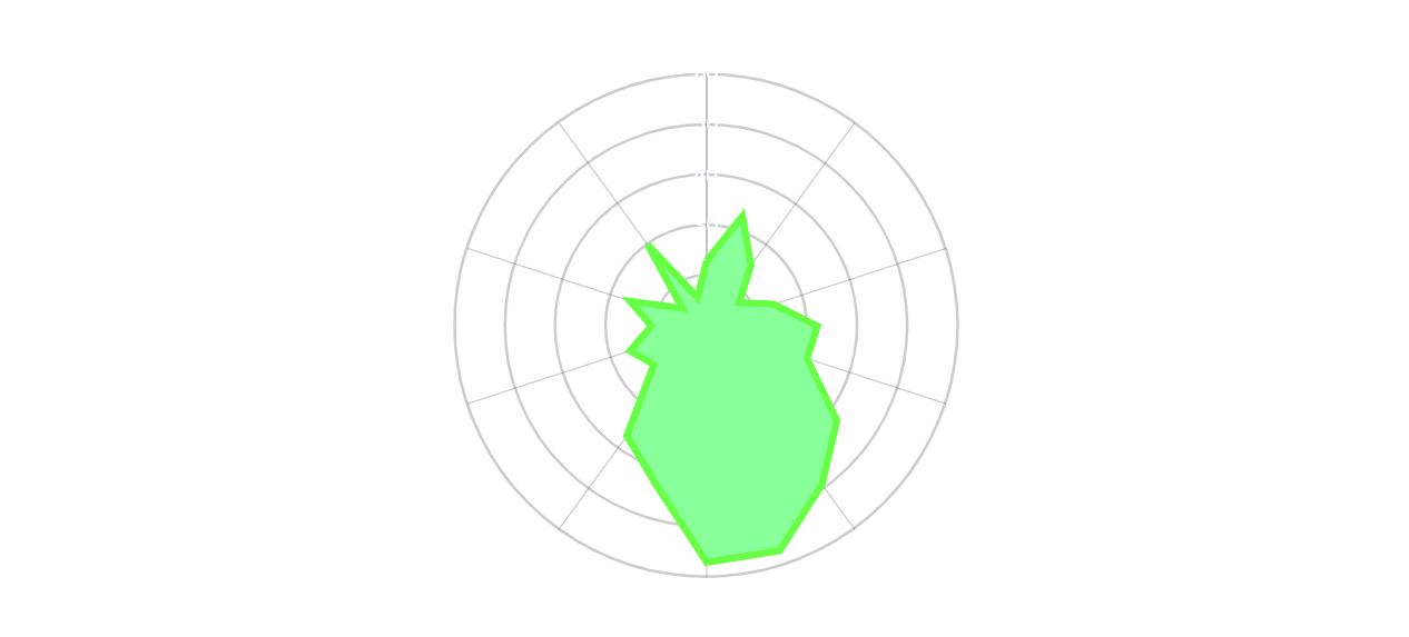
This just touches the absolute minimum of possibilities. Read the AMCharts docs for more info.
Remember that the output of the query is not a graph, but a JSON object that describes the graph. Some parts of the LRS can send the results of the query to the renderer transparently. For instance, when you place a custom block on VQL on a dashboard, it's rendered automatically. However, some uses of VQL just return the result to you. In that case, you can use our client library to render the result. Note that calling on our client library does not send the data to our servers, it just pulls in some logic into your code.
In your html, add the following line
<script src="https://lrs.io/integrations/public/vqlUtils/renderer.js"></script>
Then, somewhere in the body, create a div and give it an ID.
<div id="chart">

</div>
vqlRender("chart", yourVQL_result, amCharts_theme_name, amCharts_theme_url, background);
This will add an IFrame to the #chart div, which pulls in our renderer. The yourVQL_result data will automatic be sent to the IFrame when it's ready to render. In the above example, you're responsible for getting the VQL result to the client. You can either run the query via AJAX, or run the query server side and template the resulting JSON into a server side HTML page render.